Example of choosing server-side hardware characteristics
Deploying 100-users 1C:DocFlow solution in Vietnam International Bank (VIB) we had to choose servers hardware characteristics for the system. We used the official 1C recommendations that can be found in this tech article. The main idea behind the article is that we can extrapolate the hardware component utilization of some live system (called Model) to our system, assuming that the model system users utilize the hardware components to the same extent as our users will.
Deploying 100-users 1C:DocFlow solution in Vietnam International Bank (VIB) we had to choose servers hardware characteristics for the system. We used the official 1C recommendations that can be found in this tech article. The main idea behind the article is that we can extrapolate the hardware component utilization of some live system (called Model) to our system, assuming that the model system users utilize the hardware components to the same extent as our users will.
The VIB project was carried out with Extended TechSupport provided by 1C, so we asked 1C experts to find a comparable 1C:DocFlow system we could use as a Model. They gave us access to hardware characteristics and hardware utilization of live 1C:DocFlow which 625 users performed approximately the same tasks our users were going to perform.
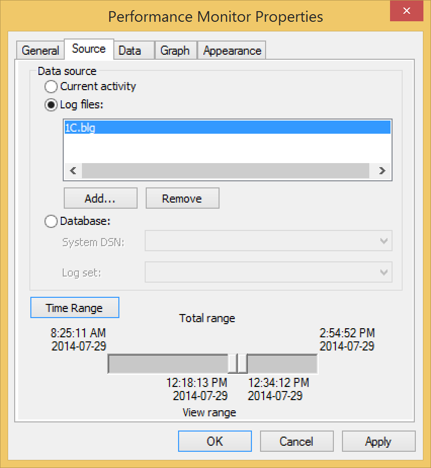
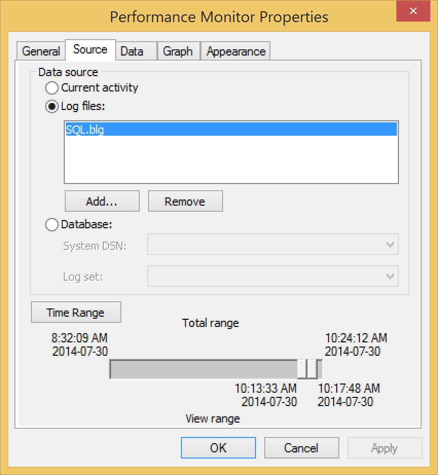
In the first place, we collected the hardware utilization counters during 2 hours of operation from 1C and DMBS servers of the Model system using Windows Performance Monitor. It gave us two files (1C.blg and SQL.blg) that can be found attached to the post.
Then we downloaded the «Calculation.xls» file and started to fill it out with the information from blg files we got. You can find our «Calculation.xls» file in the attachment.
First of all, we put the number of active users for the Model system (625) and for our system (100).
To be on the safe side we chose the interval of the highest hardware utilization rate and used counters measured on these intervals.
The number of 1C and DBMS servers CPU cores of the Mode system was 16 and 24 correspondently. Average of “%Processor time” counter for the 1C server on the interval we chose was 46.45%.
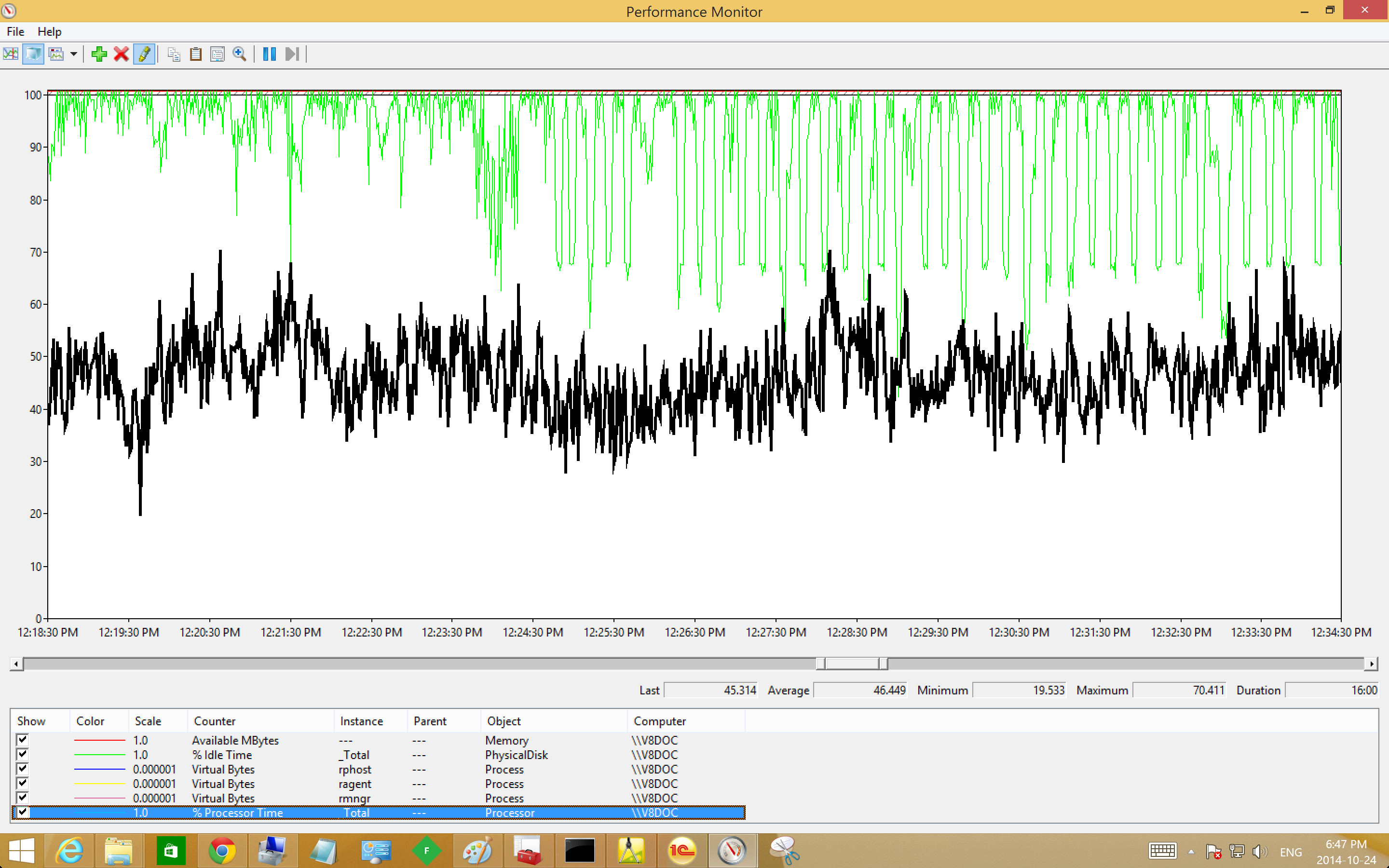
Excel formula automatically calculated the number of CPUs we needed for the 1C server of the target system: 1.19. The formula is quite simple and thoroughly explained in the tech article mentioned above. Long story short, our system is going to utilize the processor 6.25 times less than the Model system (625/100). The Model system utilizes 46.45% of 16 cores, which is equivalent to 100% utilization of 7.432 CPUs (46.45*16/100). Therefore our system is going to fully utilize 1.19 CPUs (7.432/6.25).
All calculations are based on the same principle, so we won’t explain them in detail down the road.
Another important thing to consider here was a processor model. 1C recommendation says we have to use a processor having at least the same one-thread performance as the Model system processor. 1C server of the Model system was built on Intel Xeon E5640 2.60 GHz whereas the data center, where we were going to rent hardware, used Intel Xeon E5-2690 2.9 GHz, which is about 2.5 times faster according to .
With all that said, we decided to allocate 2 virtual cores for our 1C server.
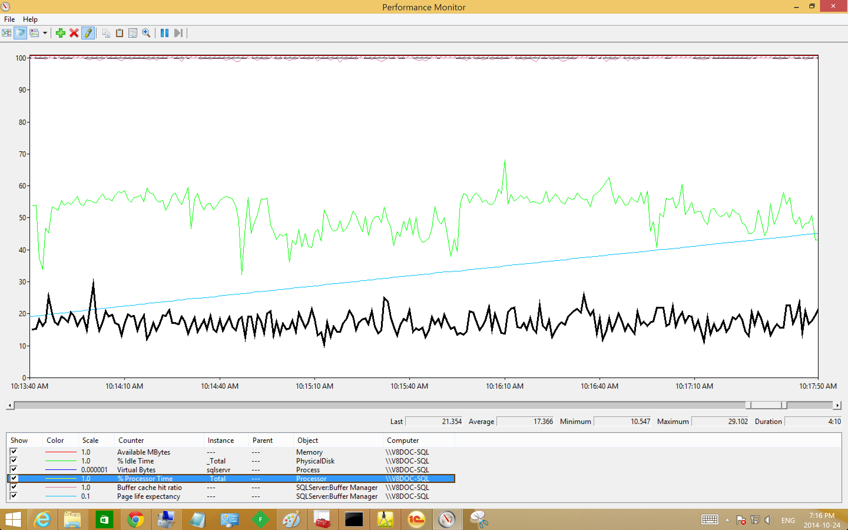
The average utilization for the SQL server processor on the interval we chose was 17.37%, which gave us 0.67 CPU cores for our SQL server.
The SQL server of the Model system used Intel Xeon E5-2630 2.3 HGz, which was about 36% slower than E5-2690. Therefore our system was going to cope with workload using only 1 core, but just to be on the safe side we decided to allocate 2 cores.
Calculating disk array performance we put “%Disk Idle Time” counters values (89% and 52% for 1C and SQL server correspondently) into the correspondent cells of the same Excel file. It gave us 10% of disk array utilization for both 1C and SQL server in sum. Therefore our system was going to suffice about one-tenth of the Model system disk array performance. Given that Model system used entry-level BM DC3500 array, we could be sure the data center’s midrange array (IBM Storwize V7000) was powerful enough for both our servers.
To calculate the RAM size for the 1C server we summed up the amount of memory allocated by all 1C server processes (ragent, rmngr and rphost) and put it into the correspondent cell of the Excel file. It gave us 3,095 Mb of memory needed for our 1C server, so we decided to allocate 4 Gb.
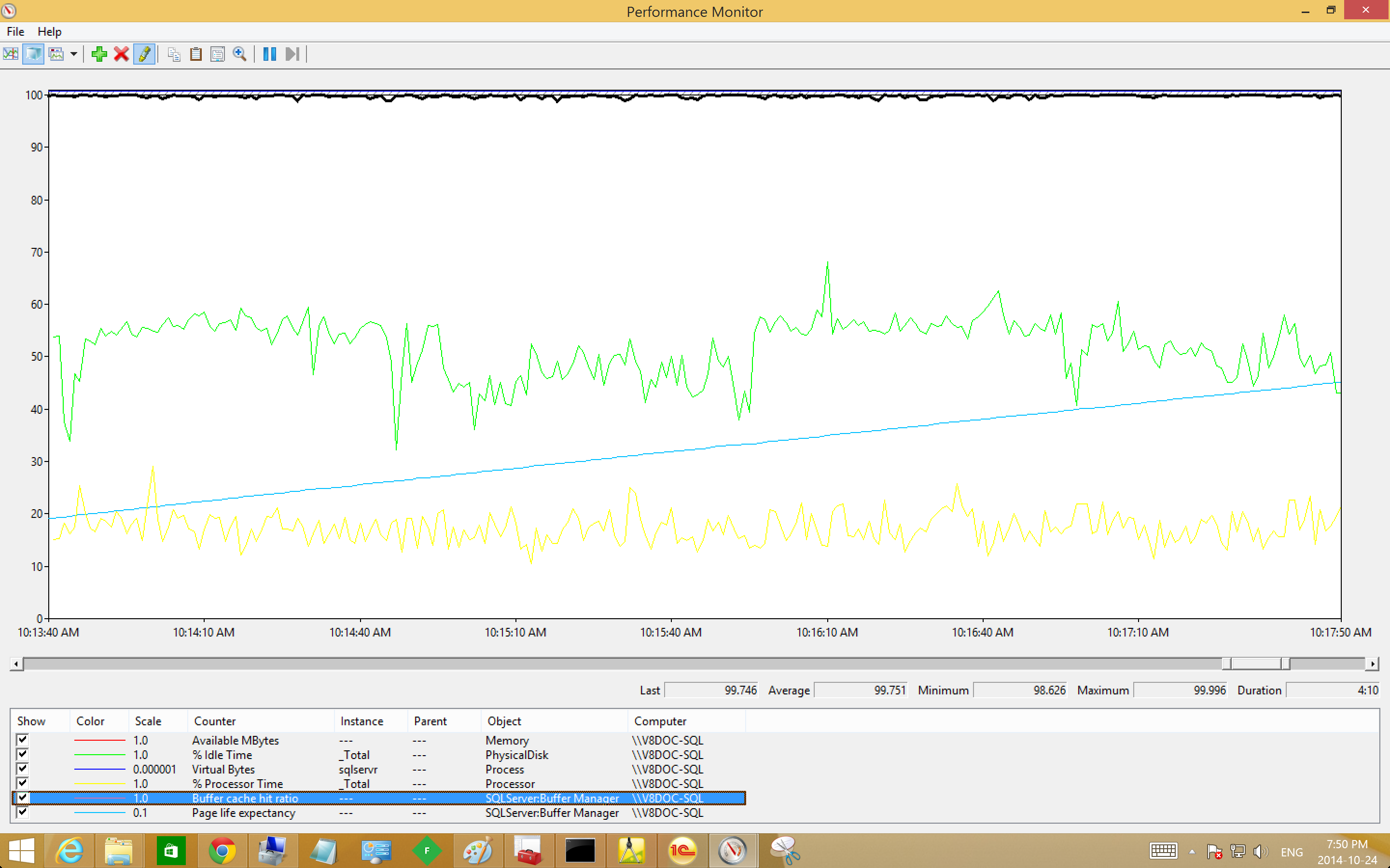
Before we could calculate the amount of RAM needed for our SQL server we had to assure the Model system SQL server doesn’t work under the memory pressure. According to 1C recommendations “Buffer cache hit ratio” counter values over 80% shows that there is no RAM shortage. In the Model system, this counter average value was 99.75%, so we could use the amount of RAM allocated by the SQL server for our calculations.
The average amount of memory allocated by sqlservr process in the interval we chose was 66,564 Mb, so we put it into the correspondent cell of the Excel table and got 12,698 Mb recommended for our SQL server and we round it up to 14 Gb.
By now, after a few months of operation, the system works well and the hardware we allocated successfully copes with the workload.

Writen by


